Background

Annie
Annie is a tech-savvy student. She uses smart devices like her iPhone and Google Home. She tends to use WhatsApp with her friends and family to share videos and links.

Annie
Annie is a tech-savvy student. She uses smart devices like her iPhone and Google Home. She tends to use WhatsApp with her friends and family to share videos and links.

One day, Annie was by her Google Home when she received a WhatsApp notification.

The advertisement contained a hidden audio attack that targeted smart home assistants.
The hidden audio was not clearly audible to Annie, but her Google Home picked up on the command. The audio could have also activated any other smart home device that is voice activated, such as smart TVs or smart washing machines.
Fortunately, the attacker did not have any malicious intentions and only used a benign command to "Play Music". In a worst-case scenario, if Annie had used a smart door lock system or alarm system, the attacker could have disabled the system to enter her home.
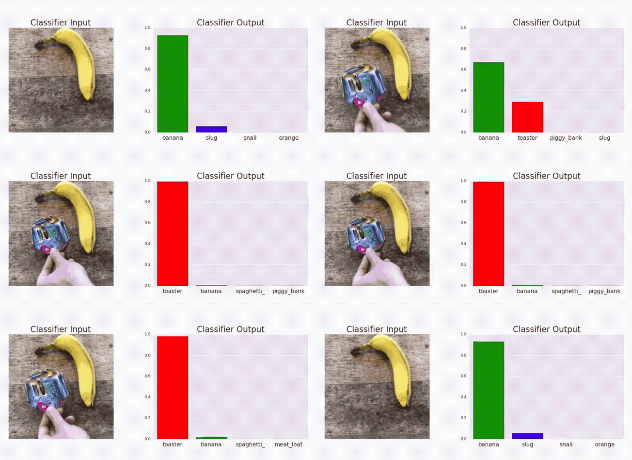
In Annie's case, she had just experience what's known as an Adversarial Attack.
Adversarial Attacks are defined as machine learning techniques intended to deceive machine learning models by supplying deceitful inputs. (Source: Wikipedia)
In the GIF above, an Adversarial Attack example was conducted by researchers who were making targeted adversarial image patches to deceive deep learning models. In this case, a banana was wrongly predicted to be a toaster due to the presence of the sticker patch.
Here, we present the two different audio clips and their corresponding waveforms.
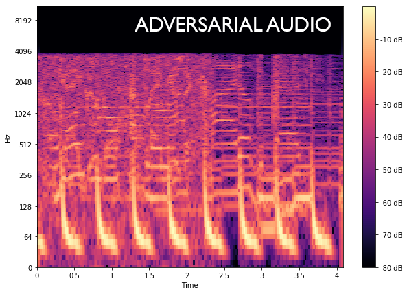
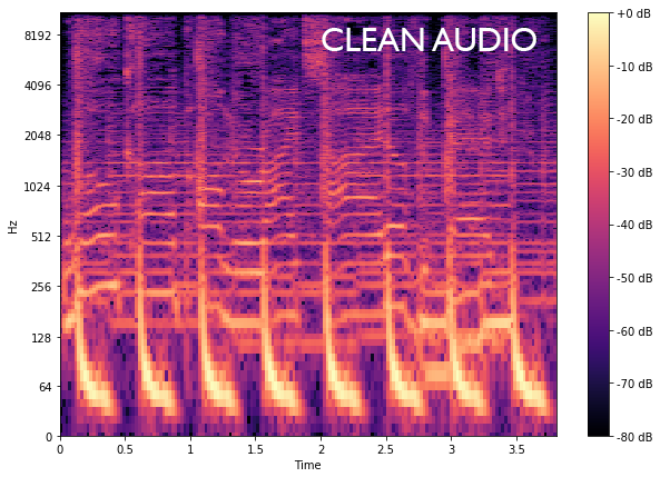
To understand the Hidden Audio attack, we can take a look at the Mel Spectrograms of both audio clips.
          import librosa
          import librosa.display
          import numpy as np
          import matplotlib.pyplot as plt

          n_fft = 2048
          hop_length = 512

          # Loading the audio
          filename1 = 'audio.wav'
          y1, sr1 = librosa.load(filename1)

          # To get absolute amplitude of the short-time Fourier Transform
          D1 = np.abs(librosa.stft(y1, n_fft=n_fft,  hop_length=hop_length))

          # Converting amplitude to decibels
          DB1 = librosa.amplitude_to_db(D1, ref=np.max)

          # Plotting mel frequency spectrogram
          plt.figure(figsize=(10,7))
          librosa.display.specshow(DB1, sr=sr1, hop_length=hop_length, x_axis='time', y_axis='log');
          plt.colorbar(format='%+2.0f dB');
A spectrogram is a visual representation of sound. The y-axis represents Frequency, the x-axis represents Time, and the colour represents the audio volume. The brightness is proportional to the volume. For example, a brighter colour means that the audio is louder. We plot the spectrograms of the audio clips on the Mel Scale, which is a scale that shows how humans can perceive the differences in tones.
